Regularly Spaced Random Events
by David Ashley
written Saturday February 11, 2023
For some experiments I was working on as a hobby I had a need for sequences
of event times where the events would occur randomly but at an average pace
of one per second. I was in a hurry so I just used an approach where I'd
build up an array of 60 random values between 0 and 60, and I'd sort them from
lowest to highest. That would give me a group of 60 random event times with an
average gap of 1 second.
Recently I wanted to dig into the problem some more, and I was wondering if
there was a simpler mechanism to generate random positive values that would
average out to 1, so I wrote a test program to generate groups of random
values as before sorted from low to high, and I'd then build up a histogram
of the gaps between each value and the next. Here is a graph of the histogram
I got:
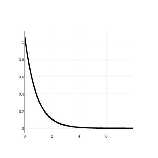
I have normalized it so the area under the curve is 1. This is a probability
density graph and to determine the probability of a gap between two values
we look at the area under the curve between those two values. For example
to determine the probability of a gap of being in the range 0 to 1 the area
under the curve ends up being about .632, so there is a 63.2% chance of the
gap between events of being up to 1 second in length.
Remember our goal is to have events average out to once per second, so the
fact that 63.2% of them are 1 second or less might seem odd. It makes
intuitive sense, however, when we consider the chance of getting a gap of
one second or more is the remainder, or 36.8%. Some of those gaps are quite
long. Suppose we get a gap of around 5 seconds. In order to balance it out we
would need 4 gaps of close to 0 seconds. Clearly we need more short gaps to
balance out the rarer long gaps.
That value .632 seemed familiar when I saw it come out of my program. It turns
out it is:

where e is Euler's number 2.71828183... but that wasn't obvious at first. I
studied the histogram and ran some tests on it and it was clear it was an example
of an exponential decay function. If I graphed the logarithm of each value
it became a straight line. That implies that starting at some maximum value
at the location were x=0 for every fixed distance we move to the right the
function's value is reduced by the same constant fraction. The general form
of such an equation is
 = k_{1}e^{-k_{2}x})
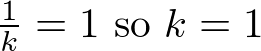
Where k1 and k2 can be adjusted to suit. At x=0 we have f(0) is equal to k1,
since raising e to the 0th power results in the value of 1. I wanted to
choose k1 and k2 such that the total area under the curve is normalized to 1,
which is the usual way probability density functions are defined. Using
calculus we know:
So if we take the definite integral from 0 to infinity it must be equal to 1:
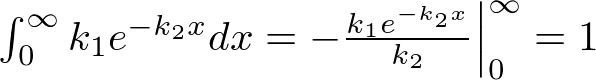
 = \frac{k_{1}}{k_{2}}=1 \textrm{ so } k_{1}=k_{2})
Interesting... we only have one constant to adjust since normalizing requires k1=k2,
so let's call our constant k. Our probability density function is now:
=ke^{-kx})
Now we want the average value to be one unit of time, so all we need to do is integrate
p(x) times x from 0 to infinity and set that to 1:
dx=\int_{0}^{\infty}kxe^{-kx}=1)
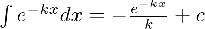
From a table of integrals or internet search we know:
+c)
Keeping in mind our exponent is negative and maintaining k positive we have:
\Big|_0^\infty=1)
\Big|_0^\infty=1)
Now in evaluating the definite integral consider evaluating where x is infinity. We have
a term that is -x which is also an infinity. But we're multiplying by e raised to a negative
infinite power, which is the same as dividing by e raised to a positive infinite power. It
should be obvious that this term goes to 0 as x goes to infinity, so the expression for
x at infinity evaluates to 0. We're left with:
=1)
Wow, what an unexpected and simple result. So our probability density function is just:
=e^{-x})
It is naturally normalized to 1. If we want to compute the probability of any period
from 0 to d we just perform a definite integral on this from 0 to d:
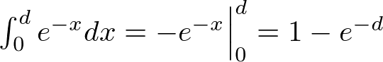
What a simple result! If we set d=1 we can evaluate this for the probability of a delay
of between 0 and 1 unit of time:

Which is the result we observed earlier.
This creates a possibility. Suppose we want to randomly generate delay values that will
average to 1 over time. We can use our equation for the probability for all values from 0
to d, only we go backwards. We generate a random value from 0 to 1 and compute what value of
d would give us that value. We then take d as the delay value:
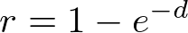
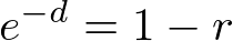
)
)
Again what a simple result! If r is a random value uniformly distributed between 0 and 1,
does subtracting it from 1 change anything? We would get another random value uniformly
distributed between 0 and 1. We can handle performing the log function on the value 1, but
if we perform it on the value 0, we get negative infinity... which is undesired. So we can
say:
, 0<r\leq 1)
We can easily generate random values from 0 to 1. The javascript function Math.random()
will generate a random value that can be 0, but it is always less than 1. In this case
we would want to subtract it from 1 to ensure we avoid the value of 0 and the log function
won't fail on us:
function randomDelay() {return -Math.log(1-Math.random());}
Here is a simple javascript test program we can use to confirm this works:
function randomDelay() {return -Math.log(1-Math.random());}
var sum=0;
var count=1000000;
var min, max;
for(var i=0;i<count;++i) {
	var d = randomDelay();
	if(i<10) console.log(d); // print out first 10 values
	if(i==0) min=max=d;
	else {
		if(d<min) min=d;
		if(d>max) max=d;
	}
	sum += d;
}
var average = sum/count;
console.log('The average delay was', average);
console.log('The minimum delay was', min);
console.log('The maximum delay was', max);
and here is a sample output:
2.0321665693865265
0.3253142574792762
0.6185181298260735
2.5320675212000734
1.6074662977335747
0.9105669018521998
2.0300596806560076
0.09811026305551855
3.473879759899842
1.5524626120886769
The average delay was 1.0011292657129276
The minimum delay was 4.3595522143325315e-8
The maximum delay was 13.602304024332579
So for this run of a million iterations the average value was within .113% of what we
expected and hoped for it to be!
It is interesting to note that over a million iterations the maximum delay we got was
only 13.6, and the minimum was practically 0. There is some probability of every
arbitrary delay, but we quickly reach the limits of numerical precision using computers.
Performing the log function on a very small number yields a large negative number, but
the odds are very small that we would randomly generate such small values.
With modern javascript on a 64 bit architecture I think the method of generating random
numbers is to compute a sequence of 128 bit random integers using bitwise operations
of XOR, AND, OR and shift, then divide by 2^128. This yields a number
that can be 0 but can't quite reach 1. If we subtract this from 1, the smallest result we can
get is 1/2^128. This would result in a delay of 88.72, since 2^128=e^88.72.
We can use this scheme to produce gaps of any desired average. If we want 20 events per
unit time, we just divide each value generated by 20. If we want an average period
of 10 units of time, we multiply each value generated by 10. We don't need to keep
track of how many events we've had so far and how much time has passed in order to
keep the algorithm honest, it automatically does that for us.
Arriving at result purely from theory
I had determined the probability density function was an exponential decay from
experimentation, and from there the results were straightforward. I had wondered
how one might determine the nature of the exponential decay from mathematical theory
but it's not at all obvious. It occured to me that the situation is very similiar
to radioactive decay of atoms. Each atom of a radioactive isotope has some nonzero
chance of decaying per unit time. When it does decay it splits apart and ceases to
exist. As such a quantity of radioactive atoms will exhibit a half life period. That
is, over some period T half of the pool will have decayed.
Our situation is equivalent to a single radioactive particle that decays at a fixed
rate but it can decay again and again forever. Our single event per unit time desired
behaviour implies that there is a time T such that there is a 50% chance an event will
have occured. We can use a value of .5 for r in our equation and compute a d value of
0.6931471805599453. That's the period for a 50% chance of getting an event. After two
such periods we would expect there is a 75% chance of getting an event, and we can
confirm our equation by using .75 for r in our equation. -log(1-.75) is 1.3862943611198906
and 1.3862943611198906/0.6931471805599453 is 2, so things are consistent.
Whatever form p(x) must have, we can define P(t) to be the definite integral
of p(x)dx from 0 to t, and it represents the odds of an event occuring within
a period t. Necessarily P(0) is 0. We know that P(2t) = 1-(1-P(t))^2 for all t.
This is because 1-P(t) is the probability that an event didn't happen
within a period t. So P(2t) would be 1 minus the chance that we didn't have an event during
period t, twice in a row, so we square the probability and subtract it from one. We also know
that P(t*n) = 1-(1-P(t))^n for t>=0 and n=0, 1, 2, 3... because for a
period t, P(t) represents the odds of an event occuring within time t, and
we can subtract that from 1 to have the odds of the event not occuring,
and by raising this to a power n we compute the probability of n periods
occuring without an event, and subtracting that from 1 yields the probability
of an event occuring within the period t*n. It turns out this equation holds true
even for non-integer n, because we can always adjust t to make n an integer if
we have to. Specifically if n is not an integer we can replace n with n' which
is the next higher integer, and then we'd replace t with t' which is t*n/n', making it slightly smaller to compensate. Now we can then consider what
happens as we let t go to zero and n be chosen such that t*n is x:
P(t*n) = 1-(1-P(t))^n
Let x=t*n
n=x/t
P(x) = 1-(1-P(t))^(x/t)
What is the limit of P(x) as t goes to 0?
P(x) represents the probability of a period occuring from 0 to x.
So certainly P(0) is 0, there is zero chance of getting a period
of exactly 0. We know that P(infinity) is 1, meaning we have a 100%
chance of getting an event within an infinite amount of time.
Clearly our function rises from 0 towards 1 at a slower and slower
rate. If we consider N(t) = 1-P(t) we have
N(x) = N(t)^(x/t) and N(0)=1 and N(infinity)=0
N(x) = (N(t)^(1/t))^x
We set k=N(t)^(1/t) and so
N(x) = k^x and all we have to do is solve for k, which must be 0<k<1
and it must converge on some value as t goes to 0.
P(x) = 1-k^x
Since P(t) was the definite integral of p(x) from 0 to t
p(x) must be the derivative of P(x) so
p(x) = -log(k)*k^x
k=e^log(k)
k^x = e^(x*log(k))
p(x) = -log(k)*e^(x*log(k))
We know 0<k<1 so log(k)<0, so we can replace log(k) with -k to get
p(x) = k*e^(-kx)
which is the same as an earlier point above and our derivation can continue
as before.
Other probability density functions
For any normalized probability density function p(x) integrating x*p(x)*dx from
zero to infinity will yield the average value. It turns out there an infinite
number of functions that will satisfy the requirements:
The average value must be 1
Values cannot be negative
Gaussian distributed numbers are almost as easy to produce as my scheme above.
Those will have an average value and a bell-curve distribution surrounding it.
This javascript function will produce Gaussian numbers with an average value
of 0 and a standard deviation of 1:
function gaussian() {
	var d, x, y;
	function rs() {return Math.random()*2-1;}
	for(;;) {
		x = rs();
		y = rs();
		d = x*x+y*y;
		if(d<1) break;
	}
	d = Math.sqrt(-2*Math.log(d)/d);
	return [x*d, y*d];
}
It works by finding a random point in the unit circle at coordinate (x,y) and
then adjusting both x and y based on the distance from the origin (0,0). We
get two kind-of independent variables. If we pick one of them and just add 1
to it we'll get a sequence that will average to 1, but it will have negative values.
We can fix this by throwing away all negative values. We can work out the probability
that we'll get a value out of the above function that is less than -1 in various ways.
A normal gaussian distribution density function is of the form k1*exp(-k2*x*x) and it
cannot be integrated to a closed-form solution, so we have to use numerical methods or
estimate the integral. It turns out about 15.9% of the time we'll get a number less than
-1. The average value of all such numbers is about -1.53. The average value of all
the remaining numbers is about .288. Combining these two balance out to 0, 15.9% of
the time we'll get an average of -1.53 and 84.1% of the time we'll get an average of .288.
We compute .159*(-1.53) + .841*.288 and the result is -.001 or so.
So we can convert our gaussian function to output values >=0 that will average to 1 by
just throwing away all values less than -1, adding 1 to each one remaining, then
multiply by 1/1.288:
function fixGaussianStep() {
	for(;;) {
		var v = gaussian()[0];
		if(v>=-1) break;
	}
	return (v+1)/1.288;
}
This is the end of the paper.
Notes on how the graph and pretty mathematical formulas were made:
File rsre-00.png: Here is the program used to generate the first graph of the histogram of
gaps between events.
Cut and paste this into
https://www.linuxmotors.com/linux/plotly/
trace1 = {
  type: 'scatter',
  x: [1.5, 2, 3, 4],
  y: [10, 15, 13, 17],
  mode: 'lines',
  name: 'Red',
  line: {
    color: 'rgb(0, 0, 0)',
    width:4
  }
};

var layout = {
  width: 512,
  height: 512
};

var data = [trace1];

var hist=[];
var bins = 1024;
var total=0;
for(var i=0;i<bins;++i) hist[i]=0;
var num = 32;
for(var i=0;i<200000;++i) {
 var a = [];
 for(var j=0;j<num;++j) a.push(num*Math.random());
 a.sort();
var scale = 8;
 for(j=0;j<num-1;++j) {
  var v = Math.floor(bins*(a[j+1]-a[j])/scale);
  if(v>=bins) continue;
  ++hist[v];
  ++total;
 }
}
var fix=bins/scale/total;
hist.forEach(function(v, ndx) {hist[ndx]=(v*fix);});
trace1.y = hist;
trace1.x=[];
for(var i=0;i<=bins;++i) trace1.x[i]=i*scale/bins;
console.log(hist[0]);
Plotly.newPlot('myDiv', data, layout);
The inline math equations were rendered dynamically on the apache web server using my own tool renderLatex.